Bris-1 mystery sample
Rev. 1/3/2023 LRM... A test case for microprobe method development for metamorphic petrology applications
Bris-1 is a random thin section that I found in the Petrology Lab when I started working as a lab manager. At the time of writing, I have no idea where it comes from. So far, it's turned out to be a garnet-bearing metamorphic rock with a lot of quartz, alkali feldspars, mica, cordierite (?), and kyanite.
Note: I use YYMMDD dates in my notes, and some of these dates may be floating around in here.
Contents
- Petrography
- Segmentation
- Major element WDS method
- P-T calculations
- Trace element mapping
- Ti-in-Quartz
- Monazite dating
- AI summary
- Maintenance
Petrography
back to top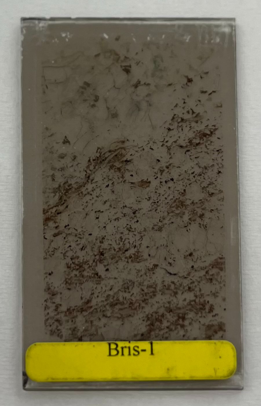
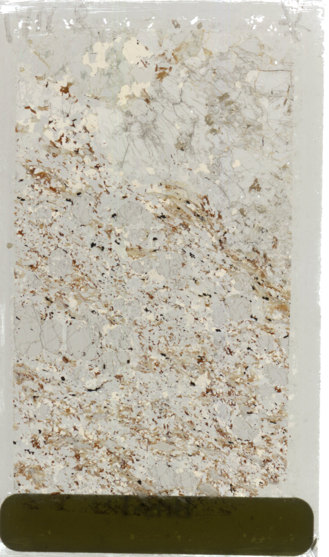
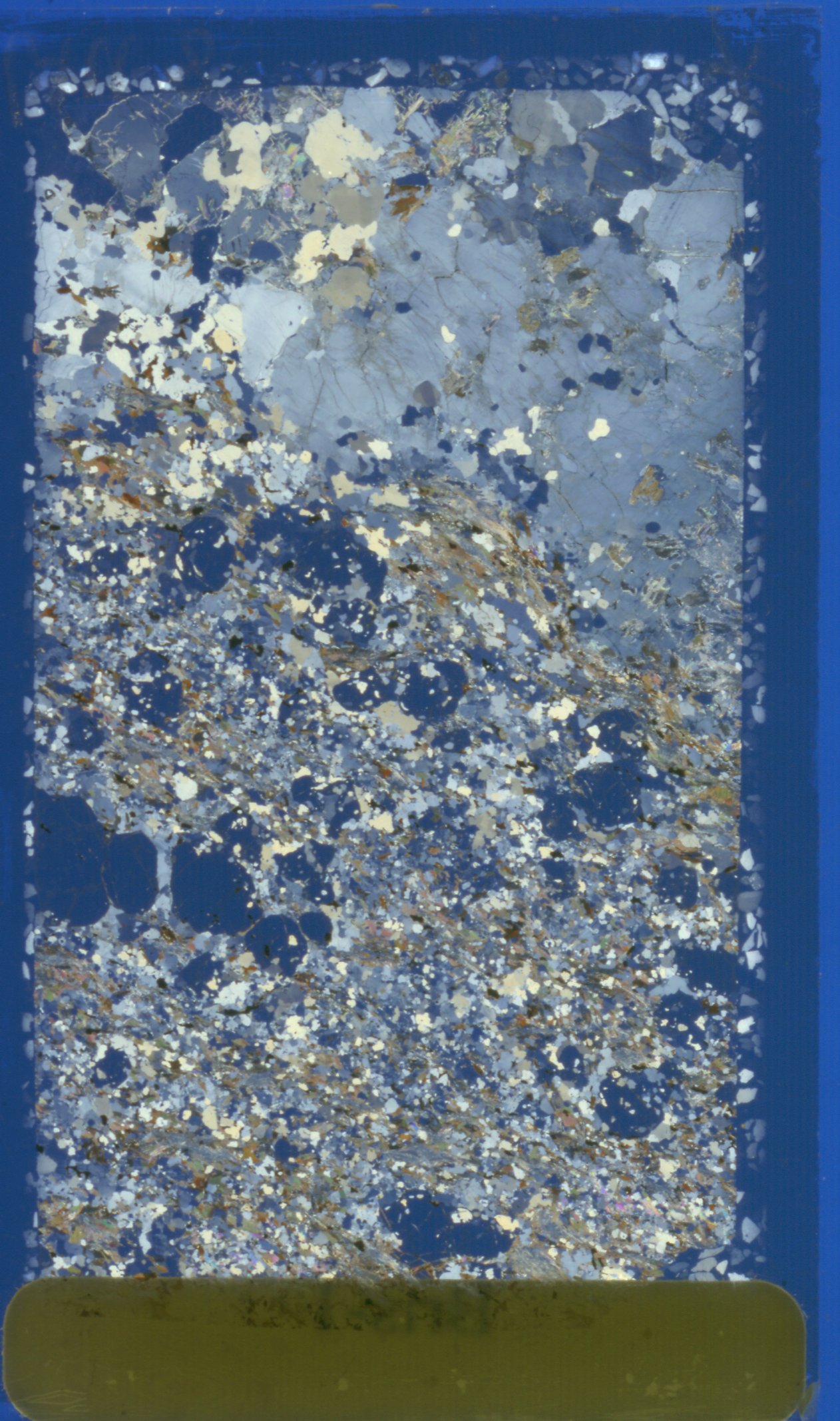
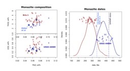
If I were a good microprobe user, I would have photographed and scanned the sample before starting any analyses, but sometimes one is in a hurry and doesn't do that. The PCA analyses, EDS analyses, and Ti-In-Qtz analyses were done before I went back to the Petrology lab to make the photo/scans.
A problem I am interested in working on is how to obtain modal mineral abundances using X-ray maps. This problem has been solved previously with various image segmentation programs including Pierre Lanari's XMapTools, but that doesn't prevent me from being curious about strategies for image segmentation or other ways to make sense of multi-channel X-ray data.
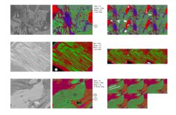
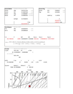
To get some preliminary X-ray data for the sample, I made a full thin section map using the following settings with the result shown below. I think it was also my intent to use the thin section to test my monazite dating method, given the elements that I had selected, but I must have forgotten about this initially as I got "sucked in" to the segmentation problem.
- 20 kV, 100 nA beam, defocused to a 20 micron circular spot
- 18.060 x 36.580 scan range with 20 micron square pixels
- 903 x 1829 pixel resolution x 20 ms dwell time = 10h 26m
- WDS: Mg(TAP), Ca(PET), Ce(PET), Mn(LiF), P(TAP)
- EDS: manually selected major elements, reduced aperture
- IMS: SED, BED-C, PCLI
At some point, I'll probably need to explain what PCA is and how it's being used here. Here are my notes about PCA:
Lowell's explanation of PCA
- The goal of PCA is dimensionality reduction. Suppose you have a dataset with many dimensions, but some of the variables are correlated. In this case, multiple variables can be summarized by simply considering a linear relationship between them.
- In geology, the use of various mineralogical indices calculated from more complete chemical analyses (e.g. Fo#, An#, Peralkalinity index) accomplishes the goal of dimensionality reduction, and is loosely analogous to PCA.
- PCA refers to a calculation that projects multidimensional data onto a new coordinate system.
- The axes in the coordinate system are mutually orthogonal, and each axis points in the direction of maximum variance.
(the "mathy" bits)
- The number of PCs is equal to the number of variables
- The PCs are unit vectors that constitute an orthonormal basis
- Note: an eigenvector is a vector "v" corresponding to a square matrix "A" such that the product A*v = lambda*v where the scalar "lambda" is the eigenvalue of eigenvector "v"
- Also note: a covariance matrix is an n x n matrix of n variables where each item in the matrix is the covariance of two corresponding variables of the variables.
- The PCs are eigenvectors of the data's covariance matrix. PCA performs a change of basis calculation to transform the original data to be expressed eigenvalues of the PCs/eigenvectors/orthonormal unit vectors.
(defining some of the jargon)
- Loading (positive/negative): refers to the degree to which a variable contributes to or is correlated with a PC
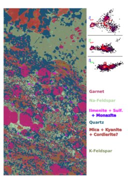
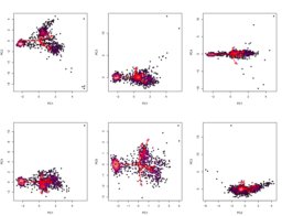
PCA was done for the Bris-1 sample in R with the image made from PC's 1, 2, and 3 mapped onto the R, G, and B channels respectively. The process of making the PCA image is extremely easy, but interpreting the colors/clusters as individual minerals and segmenting the image into the clusters is difficult.
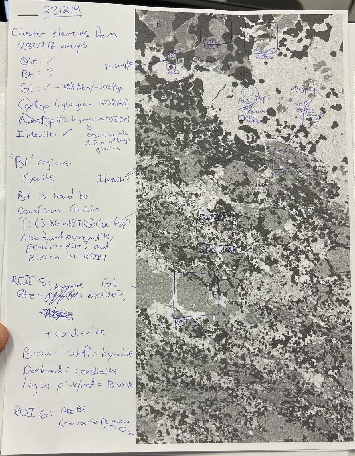
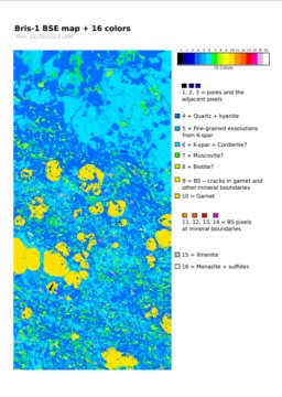
After looking around with the EDS, here are the main takeaways (with colors in reference to the PCA image above):
- The quartz, garnet, and ilmenite seem to have been identified correctly.
- I misidentified the feldspars: the lighter green phase is a Na-rich feldspar (~75% Albite), and the darker green phase is a K-rich feldspar (~90% Orthoclase).
- In the patchy red/orange/brown areas that I labeled as "Biotite?" several minerals are present:
- Yellowish-brown = Kyanite
- Dark red = Cordierite
- Light pinkish-red = Biotite
- Darker maroon =
also biotite, containing Ti?fine-grained kyanite + quartz
- Also, it seems like there could be two micas growing together: a more K-rich mica, and a more Fe+Ti-rich mica (biotite and muscovite?).
- The light pink/purple color seems to include both monazite and sulfides (pyrrhotite?) as well as ilmenite.
- The white phase marked as "Sulfides?" is actually apatite.
Segmentation
back to topHere's what I've tried so far with regards to segmentation:
- K-means clustering EDS maps in ImageJ
- "Segmenting" images (to visualize potential clusters) using PCA in R + ImageJ
- K-means clustering EDS maps in R
- Naively segmenting BSE images using the "16 colors" LUT in ImageJ
- Staring at transmitted light photomicrographs wishing that the thin section would just segment itself
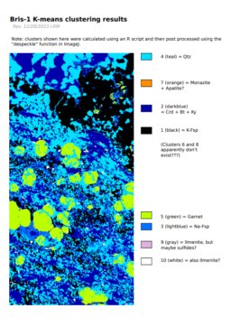
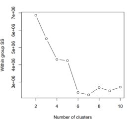
To evaluate the effectiveness of the K-means clustering approach, I need a way to "ground truth" the phase proportion, and I can't think of a better way to do this than point counting. To count points, I wrote a basic R script (240102) to randomly display a 100 x 100 pixel subregion of the PC image shown above, and used this to count ~120 points at the center of each sampled region. I then compared this result to the proportions of the clusters which are shown in the image above.
Here is a table of the point counting results:
| phase_options | phase_props | n_counted |
|---|---|---|
| Quartz | 0.49 | 49 |
| K-spar | 0.18 | 18 |
| Na-Spar | 0.05 | 5 |
| Garnet | 0.12 | 12 |
| Biotite | 0.05 | 5 |
| Kyanite | 0.08 | 8 |
| Cordierite | 0.02 | 2 |
| Ilmenite | 0 | 0 |
| unclear | 0.01 | 1 |
Here is a table of the K-means clustering results:
| cluster_id | cluster_names | prop_clust | n_clust |
|---|---|---|---|
| 1 | K-fsp | 0.238427 | 393783 |
| 2 | Crd+Bt+Ky | 0.222723 | 367846 |
| 3 | Na-Fsp | 0.078168 | 129102 |
| 4 | Qtz | 0.352312 | 581874 |
| 5 | Grt | 0.098683 | 162984 |
| 6 | none_6 | 0.000000 | 0 |
| 7 | phosphate | 0.000455 | 751 |
| 8 | none_8 | 0.000000 | 0 |
| 9 | Ilm+Sf | 0.001321 | 2181 |
| 10 | Ilm+Sf2 | 0.007911 | 13066 |
...so not great, but not terrible? My guess is that the proportion of quartz is being underestimated by the K-means clusters because the clustering algorithm can't separate fine-grained quartz that is intergrown with other stuff (e.g kyanite) from the big quartz grains.
Major element WDS method
back to top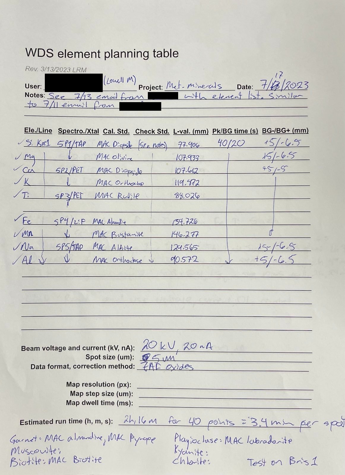
My notes about reporting uncertainty:
Uncertainty is going to depend on these factors:
- Counting statistics (more X-ray counts per second means more precision)
- Quality of standards (are the reported concentrations accurate? are the standards homogeneous?)
- Instrumental drift (were there any big temperature swings in the lab?)
- User error and sample preparation (were any mistakes made preparing the sample, applying a conductive C coating, doing the calibration, or performing the analyses?)
What I would recommend is that if some of the standards were analysed in replicate as unknowns, then the user could say something like "uncertainty was estimated based on the standard deviation of N replicate analyses of [a diopside standard (or whatever)] provided by the microprobe lab." Alternatively, if this wasn't done, or if the user feels like there weren't any major problems based on periodically analyzing one of the standards as an unknown, then the user can just report the errors from counting statistics.
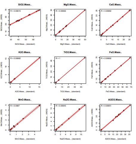
To check the precision/accuracy of the quantitative method, I analyzed a bunch of replicates of some of my reference materials to create calibration-curve-like plots and calculate a regression line and uncertainty envelope. It seems like this is probably the most robust way to estimate all of the sources of uncertainty including user error and quality of the standards.
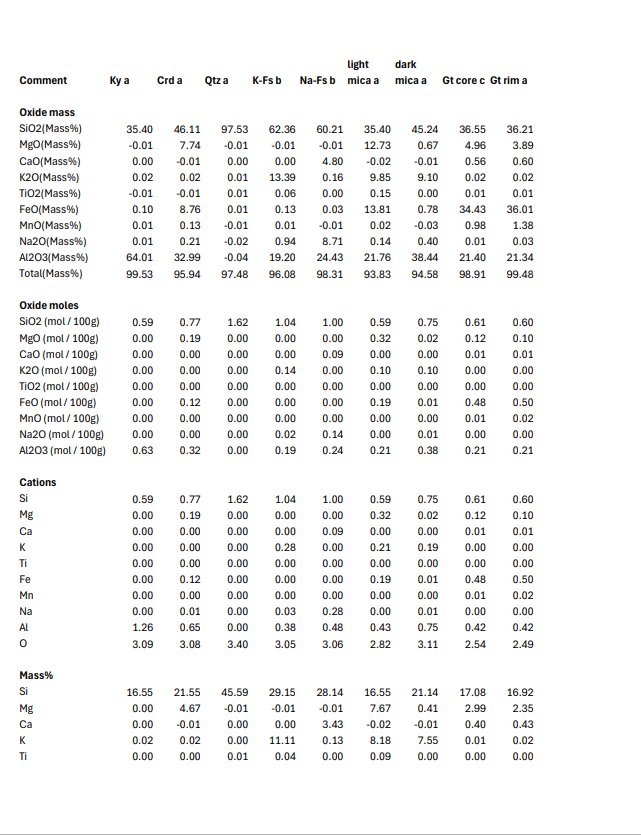
Some of the textures were so complicated/fine scale that I "threw up my hands" and decided to just collect some quant maps. I wrote a little R script to retrieve selected pixels from the stack of CSV files produced by the microprobe software using a .png image created for each phase, which I "painted" white in ImageJ to manually identify the pixels of interest. An added benefit of this approach is that the short dwell time eliminates beam damage affecting some of the micas and maybe also the alkali feldspars. This method worked surprisingly well. There were some issues with contamination between pixels and there was a little stage offset between mapping passes (6 total, with two "rows" of elements with two background points for each).
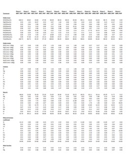
Garnet trace element maps
back to top
Most users are unsure about the best conditions to use for mapping trace elements. Usually the trace element in question is Yttrium, and the material in question is garnet. Ideally, I should be able to provide a general way for the user to figure this out independently without wasting a bunch of time trying things randomly, and collecting a few "qualitative" WDS spectra to test out different spectrometer/element pairings, dwell times, and beam conditions seems like the best way to do this. I've written about this process elsewhere.
The figure above shows the results of a basic test that I did, which basically determined -- without making any maps ahead of time -- that mapping Y, Ti, Sc, and Cr would be a waste of time for this garnet for the amount of time that I was prepared to spend doing so.
Ti-in-Quartz
back to topOne method I have been working on is quantifying Ti in quartz, which seems to be a popular thermobarometer these days. This is obviously challenging because one doesn't think of quartz as containing a lot of Ti, but it's also challenging because of some "manual labor" that goes into summing the counts collected on multiple spectrometers.
P-T calculations
back to topI know literally nothing about thermobarometry in metamorphic rocks. Or really about any rocks. Here's some literature I've found:
-
Caddick & Thompson (2008) -- Perplex models were used to evaluate the accuracy of different commonly-used mineral
thermobarometers as a function of mineral assumblages/whole rock compositions:
- X-FeMg for Garnet+Biotite -- their equations 1 and 2
- X-Ca for Garnet+Plagioclase -- their equation 4
- Stormer (1975) -- Classic two-feldspar thermobarometer
- Thomas et al. (2010) -- Ti-in-Qtz paper
Here's what's worked so far: If I use the Garnet-Biotite Mg-Fe exchange and the Garnet-Plag Ca exchange thermobarometers together, I get ~820 C at 1 GPa. If I try to use the two-feldspar thermometer, I get something around 480 C, but I think I can explain this by saying pointing out that the very low Na concentration is outside the compositional range where this model is valid. I haven't been able to get the Ti-in-quartz thermometer to work in Excel in a way that reproduces the figure from Thomas et al, but according to the figure, I should get P-T conditions that agree with the Bt+Plag+Bt thermometers around 750C. However, I'm not totally sure about the a-TiO2 term as I haven't seen much rutile in the sample. Is the one grain evident from my quant maps actually in equilibrium with the quartz?
Monazite dating
back to top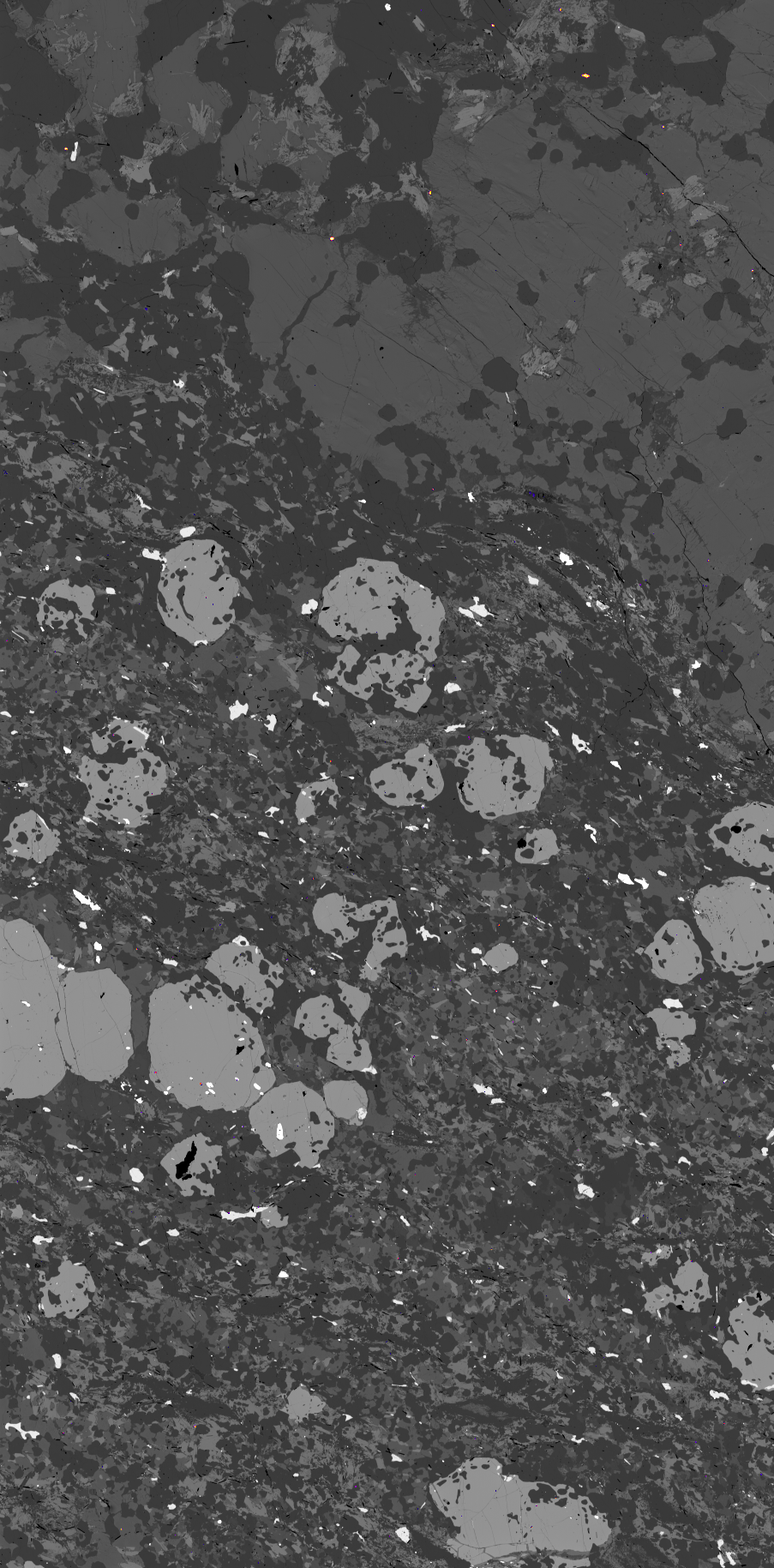
Aside: Here is my method formaking the overlay image for future reference:
- Open the "COMPO" and "Ce" maps in ImageJ
- Select the "Ce" image and click "Image > Adjust > Threshold..." to open the thresholding tool
- Choose the pixel range going from some arbitrary minimum value up to the maximum value so that only the most Ce-rich pixels are selected, and close the menu without clicking any buttons. At this point, the chosen pixels should appear red on the image.
- Click "Edit > Selection > Create Selection" to select the hilighted pixels
- Click "Image > Lookup Tables > Fire" to apply a lookup table
- Click "Image > Type > RGB Color" to change the now false color image to RGB format
- Ctrl+C to copy the selected pixels
- Select the "COMPO" image, and click "Image > Type > RGB Color" to change it also to RGB format
- Ctrl+V to paste the selected pixels onto the "COMPO" image
- Zoom in on a bright area and double check that the pasted pixels are in the right location. Fortunately, you can click and drag the pasted pixels if they need to be adjusted. I suspect that the they will be accurate if the maximum area of the selection matches the maximum area of the image, but not if the area is smaller.
- At this point, you're done. Save the image in the desired format (e.g. as a RGB-formatted .bmp file).
231229 Summary of monazite compositions and calculated U-Pb dates. Looks like the Bris-1 monazites are about 120 Ma younger than the USGS 44069 ones, which suggests an age of about 300 Ma.
Dark blue X's = USGS 44069 monazites from the Wilmington Complex with a SHRIMP age of 424 Ma. Red X's = Bris-1 sample. Light blue circles = representative EPMA compositions for USGS 44069 reported by Didier et al. (2017; Table 1), which yield a calculated age of about 330 Ma.
Dating the monazites was pretty straightforward: the calibration process took about an hour, and the analyses took about 5 minutes each.
AI summary
back to top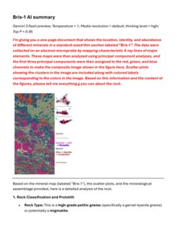
260115 -- When I started working on this page, AI was not a thing. Now it is, and I've used Google's "Gemini" model in Google AI Studio to interpret the PCA image and some major element data. The goals of this exercise were to see if the AI could describe the petrology of the sample and determine the location where the sample may have been collected. I don't feel confident in my ability to properly evaluate the results, so make of this what you will!
Maintenance
back to topTODO
- Add accuracy and precision estimates for 20 kV quant method.
- Add monazite images showing zonation and analysis locations. (photo of notes)
- How do EDS maps compare to my full thin section map? Need to include some EDS maps and spectra for comparison.
- How do the Ti concentrations compare to the CL brightness?
- Are any other elements zoned in the garnet?
- Are there any other zoned minerals in the sample?
- Would segmentation work better if I try remapping it with more major elements on the WDS? (WDS:Si,Al,Ca,Fe,Mg + COMPO)
- How quickly can I make a nice quality full thin section map?
- Add residual plots to R script that makes major element calibration curves
- Is my aluminosilicate actually Kyanite (or is it sillimanite? or Andalusite?)
- Add statistical criteria for trace element maps from my notes in Google Docs
Bugs
- Top row should be repeated on my print composition tables
- Add some space between phase id images on my quant map figure
- Need to upload R script for extracting quant map pixels to GitHub